Introduction

Theory

Notation

The notation throughout this document is mostly consistent with papers from the Darden group. Because complex numbers are used, we choose \(A,B\) to label atoms. The coefficients, e.g atomic charges for electrostatics or \(C_6\) coefficients for dispersion, are denoted \(C\). Similarly to Darden, we use \(1,2,3\) to label the three axes of the lattice vector.

Basic overview

We are interested in systems whose energy is defined by a pairwise summation for a given configuration, \(\mathbf{r}\):

(1)\[U(\mathbf{r}) = \frac{s}{2} \sum_{A \ne B} \frac{C_A C_B} {\left|\mathbf{r}_A - \mathbf{r}_B\right|^p}, \quad p>0,\]

where \(s\) is a scale factor to convert the result to the correct units, e.g. the Coulomb constant \(\frac{1}{4 \pi \epsilon_0}\) commonly encountered in electrostatic calculations. We can extend eq. (1) to a periodic system by introducing the three lattice vectors \(\{\mathbf{a}_1, \mathbf{a}_2, \mathbf{a}_3\}\) and summing over image cells \(\mathbf{n} = n_1 \mathbf{a}_1 + n_2 \mathbf{a}_2 + n_3 \mathbf{a}_3\) indexed by the integers \(\{n_1, n_2, n_3\}\):

(2)\[U(\mathbf{r}) = \frac{s}{2} \sum_{\mathbf{n}^*} \sum_{A,B} \frac{C_A C_B} {\left|\mathbf{r}_A - \mathbf{r}_B + \mathbf{n}\right|^p}, \quad p>0,\]

The asterisk over the summation in (2) is to emphasize that the \(A=B\) term is omited for the home box (\(\mathbf{n}=\mathbf{0}\)) to avoid self interaction. This brute for summation is slowly convergent for low powers of \(p\), and in three dimensional space is conditionally convergent (i.e., the result depends on the order of summation and thus the macroscopic shape of the crystal) for \(p<4\). Even the dispersion term of the Lennard-Jones potential, which has \(R^{-6}\) decay, suffers truncation artifacts due to the fact that all terms are attractive, reducing the scope for error cancellation.

The Ewald method overcomes these difficulties by taking a single slowly, and perhaps conditionally, convergent summation and turning it into two rapidly and absolutely convergent series. A complete derivation of Ewald summation is beyond the scope of this document, but we will highlight some salient features of the method.

In one dimension, the density due to particles we are interested in can be represented as a delta function. At each point we can subtract a Gaussian function with exponent \(\kappa\), effectively shielding the delta function, making it shorter ranged and thus reducing the number of interactions it will be involved in; this is shown in Figure 1.. The Gaussians are then added back in with the opposite sign as a separate term; this constitutes a smooth, periodic function that is amenable to modeling with trigonometric functions. Using a tight Gaussian for screening will result in effective cancellation of the delta function, requiring very few summations for the first term, however many trigonometric functions will be needed to model the second term properly, due to its spiky features. Conversely, a diffuse Gaussian will be ineffective at shielding the delta functions, requiring more terms in the first summation, but the smooth nature of the Gaussians will require few trigonometric funtions to describe the second term. In this document, we refer to the Gaussian’s diffuseness \(\kappa\) as the attenuation parameter.

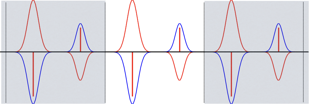
Figure 1. Depiction of the one dimensional density along a line for a system comprising two particles – one with a negative coefficient and the other positive. The primary unit cell in the center is flanked by image cells. The red lines show the original density as delta functions, with the Gaussian screening density subtracted off, to form the total short range density. The blue lines show the Gaussian screening density that is added back in, defining the long range density.

We can translate these arguments about the density, \(\rho(R)\), into methods for evaluating the potential, \(\phi(R)\), using Poisson’s equation:

(3)\[\nabla^2 \phi(R) = -\frac{\rho(R)}{\epsilon_0}.\]

This yields an identity for the kernel used to generate the potential:

(4)\[\frac{1}{R^p} = \frac{f_p(R)}{R^p} + \frac{1 - f_p(R)}{R^p}.\]

where we introduced the shorthand \(R = \left|\mathbf{R}\right| = \left|\mathbf{r}_A - \mathbf{r}_B + \mathbf{n}\right|\). This is the starting point for the detailed derivation of Ewald summations provided by [Wells:2015:3684], to which we refer the interested reader. The convergence function used in (4) is

(5)\[f_p(R) = \frac{\Gamma\left(\frac{p}{2}, \kappa^2 R^2 \right)}{\Gamma\left(\frac{p}{2}\right)}.\]

with the numerator defined by the upper incomplete gamma function

(6)\[\Gamma\left(n, x \right) = \int_x^\infty t^{n-1}e^{-t} \mathrm{d}t = 2\int_{\sqrt{x}}^\infty u^{2n-1}e^{-u^2} \mathrm{d}u,\]

while the denominator involves the gamma function

(7)\[\Gamma\left(n\right) = \int_0^\infty x^{n-1} e^{-x}\mathrm{d}x.\]

For the Coulomb case, whose kernel is \(\frac{1}{R}\), the function \(f_p(R)\) is the complementary error function, and the resulting decomposition is plotted in Figure 2..

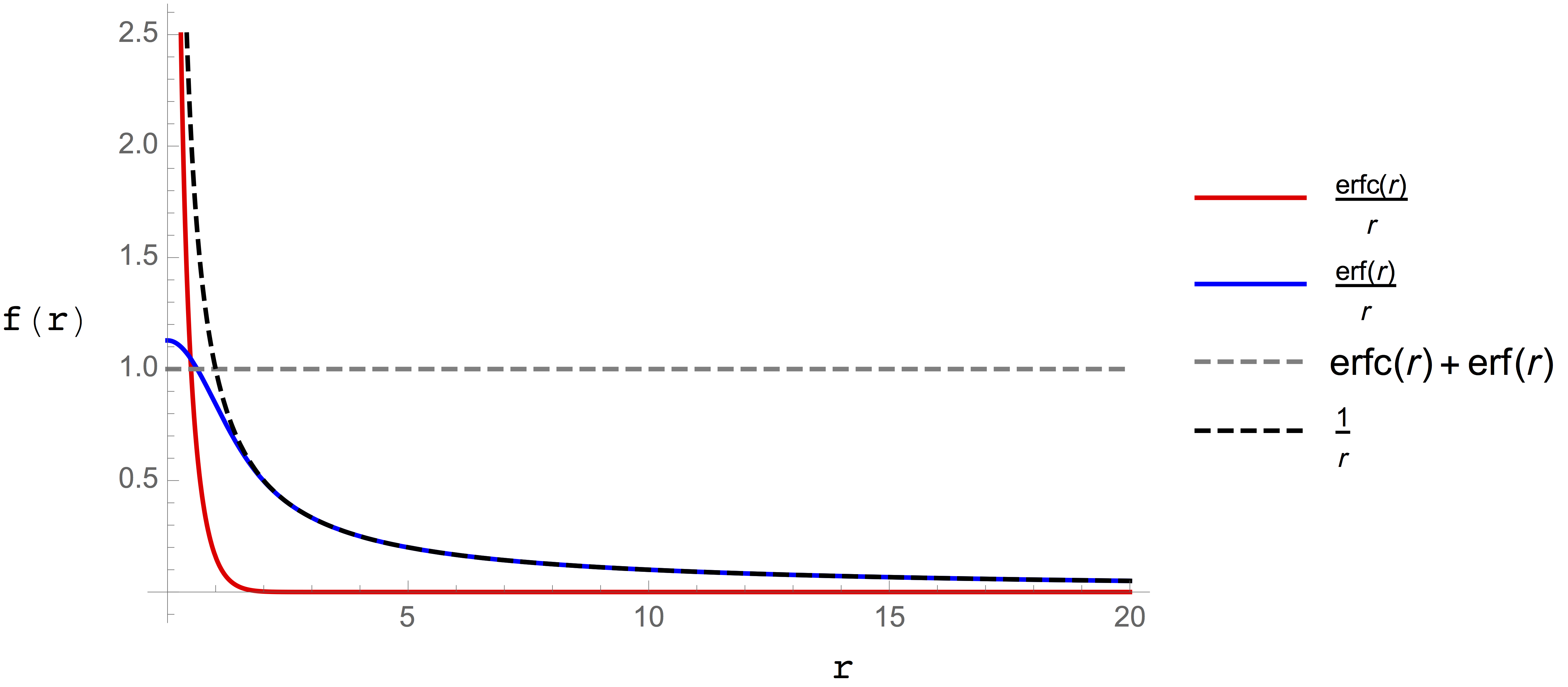
Figure 2. Decomposition of the Coulomb potential (black dashed line) into short range (red line) and long range (blue line) terms. The dashed gray line shows that the sum of the two terms is gives a numerator of one, proving that this decomposition is exact.

The short ranged term (red line) decays rapidly and is thus well suited to evalution with pairwise summation using a short cutoff. The long ranged term (blue line) is free from singularities, but still has the long tail that causes the convergence issues so another approach is needed. We’ve already noted that trigonometric functions are likely to be well suited to describing the density associated with this term. Moreover, given that

(8)\[\frac{\partial}{\partial x} e^{i\mkern1mu x} = i\mkern1mu e^{i\mkern1mu x}.\]

introducing exponentials will turn the problematic \(\nabla^2\) term in (3) into a constant, making the equation trivial to solve. In light of Euler’s formula

(9)\[e^{i\mkern1mu x} = \cos(x) + i\mkern1mu \sin(x)\]

we can introduce the aforementioned trigonometric basis and the exponentials using the Fourier transform:

(10)\[F(t) = \int_{-\infty}^{\infty} f(x) e^{-2 \pi i\mkern1mu x t} \mathrm{d}x.\]

A full derivation can be found in [Wells:2015:3684] so we will provide only the results here. Evaluation of the long-range term requires the introduction of reciprocal lattice vectors, \(\{\mathbf{a}_1^*, \mathbf{a}_2^*, \mathbf{a}_3^*\}\), defined in terms of the unit cell’s lattice vectors \(\{\mathbf{a}_1, \mathbf{a}_2, \mathbf{a}_3\}\) as

(11)\[\mathbf{a}_\alpha^* \cdot \mathbf{a}_\beta = \delta_{\alpha\beta}, \quad \alpha,\beta \in \{1,2,3\}\]

to obtain the correct integration range in the Fourier transforms. This ‘reciprocal space’ treatment uses notation for summation over reciprocal lattice vectors, \(\mathbf{m}\), analogous to that used for summation over real space lattice vectors: \(\mathbf{m} = m_1 \mathbf{a}_1^* + m_2 \mathbf{a}_2^* + m_3 \mathbf{a}_3^*\), with integers \(\{m_1, m_2, m_3\}\). With these definitions in hand, we can define the structure factors needed throughout the reciprocal space treatment, which come from the discrete Fourier transform of the density:

(12)\[S(\mathbf{m}) = \sum_A C_A e^{2 \pi i\mkern1mu \mathbf{m} \cdot \mathbf{r}_A}\]

It is in the evaluation of the structure factor where traditional Ewald and particle mesh Ewald approaches differ. In traditional Ewald summation, (12) is evaluated as written; this requires \(\mathcal{O}(N) \mathbf{m}\) vectors and \(\mathcal{O}(N)\) terms in the summation, resulting in \(\mathcal{O}(N^2)\) overall cost. It is worth noting that this can be reduced to \(\mathcal{O}(N^{\frac{3}{2}})\) with judicious choice of attenuation parameter [Perram:1988:875].

In 1993, Darden and co-workers [Darden:1993:10089] realized that the discrete Fourier transform of the density, could be performed using the \(\mathcal{O}(N\log(N))\) fast Fourier transform (FFT) algorithm if the atoms were arranged in a perfectly uniform mesh. To make the method general, they used spline interpolation to evaluate the density on a mesh, which allows the potential to be evaluated on that mesh using FFTs. The potential at each atomic center can then be extracted from the mesh using the exact same interpolation scheme. The smooth PME method [Essmann:1995:8577] introduced cardinal B-Splines for the interpolation; these can be analytically differentiated using a trivial recursion scheme, allowing derivatives of the potential, and therefore forces, to be trivially computed.

Working equations

The partitioning introduced above results in a short-range direct space energy \(U_\mathrm{dir}\) that is evaluated using standard pairwise loops, and the reciprocal space energy \(U_\mathrm{rec}\) that is evaluated via FFTs. The \(U_\mathrm{rec}\) term inextricably interacts each atom with all atoms, including itself. In light of the restriction in the summation of (2), this is not physical and this self interaction is removed by adding the \(U_\mathrm{slf}\) term. Certain terms have specific classes of interactions neglected, e.g. 1-2 interactions in electrostatics, to decouple electostatic and bond stretching terms; a masking list \(\mathcal{M}\) comprises these excluded pairs. The reciprocal space contribution present for such interactions is removed by addition of the \(U_\mathrm{adj}\) term.

A few conventions exist in normalizing the Fourier transform; to be consistent with the works of Darden and co-workers [Essmann:1995:8577], we use the definition in (10), which differs from that used in [Wells:2015:3684] by a factor of \(2\pi\) in the plane waves. Consequently, our derivation and implementation uses the identity

(13)\[e^{-a^2 x^2} = \frac{\sqrt{\pi}}{\kappa} \int_0^\infty e^{-\frac{\pi^2 m^2}{\kappa^2}} e^{-2 \pi i\mkern1mu m x} \mathrm{d}m,\]

in contrast to Wells et al.’s use of

(14)\[e^{-a^2 x^2} = \frac{1}{2\kappa\sqrt\pi} \int_0^\infty e^{-\frac{m^2}{4 \kappa^2}} e^{-i\mkern1mu m x} \mathrm{d}m\]

to expand three dimensional Gaussians. The result is that every reciprocal space term involving incomplete gamma functions should be multiplied by \((2\pi)^{p-3}\) and we define the quantity \(b\) as \(\frac{\pi m}{\kappa}\) instead of \(\frac{m}{2 \kappa}\).

With these preliminaries out of the way, we can show the energy expressions, and derivatives thereof.

Potential Expressions

(15)\[\phi_\mathrm{dir}\left(\mathbf{r}_A\right) = \frac{s}{\Gamma\left(\frac{p}{2}\right)} \sum_{\mathbf{n}^*} \sum_{B \notin \mathcal{M}} \frac{\Gamma\left(\frac{p}{2},\kappa^2 R^2 \right) C_B} {R^p_{\vphantom{P}}}\]

(16)\[\phi_\mathrm{adj}\left(\mathbf{r}_A\right) = \frac{s}{\Gamma\left(\frac{p}{2}\right)} \sum_{B \in \mathcal{M}} \frac{\left[\Gamma\left(\frac{p}{2},\kappa^2 R^2 \right) - 1 \right] C_B} {R^p_{\vphantom{P}}}\]

(17)\[\phi_\mathrm{rec}\left(\mathbf{r}_A\right) = \frac{\pi^{p-\frac{3}{2}}_{\vphantom{P}} s} {\Gamma \left(\frac{p}{2}\right) V} \sum_{\mathbf{m} \ne \mathbf{0}} \frac{\Gamma \left(\frac{3-p}{2},\frac{m^2 \pi ^2}{\kappa ^2}\right)} {m^{3-p}_{\vphantom{P}}} S(\mathbf{m}) e^{-2 \pi i\mkern1mu \mathbf{m}\cdot\mathbf{r}_A}\]

(18)\[\phi_\mathrm{slf}\left(\mathbf{r}_A\right) = -\frac{\kappa^{\ p}_{\vphantom{P}} s} {p \Gamma\left(\frac{p}{2}\right)}C_A\]

The notation \(B \notin \mathcal{M}\) in (15) denotes that all pairs are included except those where \(\mathbf{m}=\mathbf{0}\) and either \(A=B\) or the pair \(A,B\) is on the masking list. Similarly, the \(B \in \mathcal{M}\) in (16) means that only those pairs on the masked list are included, and only the \(\mathbf{m}=\mathbf{0}\) term is considered. In (17) we use the volume \(V = \mathbf{a}_1\cdot\mathbf{a}_2\times\mathbf{a}_3\) and the scalar \(m = |\mathbf{m}|\).

Energy Expressions

(19)\[U_\mathrm{dir} = \frac{s}{2 \Gamma\left(\frac{p}{2}\right)} \sum_{\mathbf{n}^*} \sum_{A,B \notin \mathcal{M}} \frac{\Gamma\left(\frac{p}{2},\kappa^2 R^2 \right) C_A C_B} {R^p_{\vphantom{P}}}\]

(20)\[U_\mathrm{adj} = \frac{s}{2 \Gamma\left(\frac{p}{2}\right)} \sum_{\mathbf{n}^*} \sum_{A,B \notin \mathcal{M}} \frac{\left[\Gamma\left(\frac{p}{2},\kappa^2 R^2 \right) - 1\right] C_A C_B} {R^p_{\vphantom{P}}}\]

(21)\[U_\mathrm{rec} = \frac{\pi^{p-\frac{3}{2}}_{\vphantom{P}} s } {2 \Gamma \left(\frac{p}{2}\right) V} \sum_{\mathbf{m} \ne \mathbf{0}} \frac{\Gamma \left(\frac{3-p}{2},\frac{m^2 \pi ^2}{\kappa ^2}\right)} {m^{3-p}_{\vphantom{P}}} S(\mathbf{m}) S(-\mathbf{m})\]

(22)\[U_\mathrm{slf} = -\frac{\kappa^{\ p}_{\vphantom{P}} s} {p \Gamma\left(\frac{p}{2}\right)}\left(\sum_A C_A^2\right)\]

For absolutely convergenct cases, with \(p > 3\), \(U_\mathrm{rec}\) has an additional term to account for the fact that the \(\mathbf{m}=\mathbf{0}\) term was erroneously excluded:

(23)\[U_\mathrm{zer} = \frac{\pi^{\frac{3}{2}}_{\vphantom{P}} \kappa^{\ p-3}_{\vphantom{P}} s} {\left(p-3\right) \Gamma\left(\frac{p}{2}\right) V} \left(\sum_{A,B} C_AC_B\right)\]

Force Expressions

(24)\[\mathbf{F}_\mathrm{dir}\left(\mathbf{r}_A\right) = -\sum_B \frac{s C_B}{R^2 \Gamma\left(\frac{p}{2}\right)} \left( \frac{p \Gamma\left(\frac{p}{2},\kappa^2 R^2 \right)} {R^{p}_{\vphantom{P}}} + 2 e^{-\kappa^2 R^2} \kappa^p \right)\]

(25)\[\mathbf{F}_\mathrm{adj}\left(\mathbf{r}_A\right) = -\sum_B \frac{s C_B}{R^2 \Gamma\left(\frac{p}{2}\right)} \left( \frac{p \left[\Gamma\left(\frac{p}{2},\kappa^2 R^2 \right) - 1\right]} {R^{p}_{\vphantom{P}}} + 2 e^{-\kappa^2 R^2} \kappa^p \right)\]

(26)\[\mathbf{F}'_\mathrm{rec}\left(\mathbf{r}_A\right) = \frac{2 \pi^{p-\frac{1}{2}}_{\vphantom{P}} i\mkern1mu s C_A} {\Gamma \left(\frac{p}{2}\right) V} \sum_{\mathbf{m} \ne \mathbf{0}} \frac{\Gamma \left(\frac{3-p}{2},\frac{m^2 \pi ^2}{\kappa ^2}\right)\mathbf{m} } {m^{3-p}_{\vphantom{P}}} S(\mathbf{m}) e^{-2 \pi i\mkern1mu \mathbf{m}\cdot\mathbf{r}_A}\]

Comparing (17) and (26), and remembering that \(\nabla_A e^{-2 \pi i\mkern1mu \mathbf{m}\cdot\mathbf{r}_A} = - 2 \pi i\mkern1mu \mathbf{m} e^{-2 \pi i\mkern1mu \mathbf{m}\cdot\mathbf{r}_A}\), we can see the relationship \(\mathbf{F}_\mathrm{rec}\left(\mathbf{r}_A\right) = -C_A\nabla_A\phi\left(\mathbf{r}_A\right)\) is obeyed, as expected. The quantity \(- 2 \pi i\mkern1mu \mathbf{m}\) is consequently the Fourier space representation of the derivative operator, and this fact leads to a trivial expresion for the forces; instead of using the regular B-Spline to interpolate the potential as we do for (17), we simply replace it with the derivative B-Spline and multiply by the coefficient posessed by the center of interest. We have to remember that this yields the forces in fractional coordinates, \(\mathbf{F}'_\mathrm{rec}\left(\mathbf{r}_A\right)\), which can be expanded to Cartesian forces using the relationship

(27)\[F_\mathrm{rec}\left(\mathbf{r}_A\right)_\alpha = K_\alpha \mathbf{a}_\alpha^* \cdot \mathbf{F}'_\mathrm{rec}\left(\mathbf{r}_A\right) \alpha \in \{1,2,3\}\]

where \(K_\alpha\) is the number of grid points in the \(\alpha\) dimension. Note that, because the positions do not appear in (22), there is no self contribution to the forces.

Virial Expressions

(28)\[\mathbf{V}_\mathrm{dir} = \frac{s}{2} \sum_{\mathbf{n}^*} \sum_{A \notin \mathcal{M}} \mathbf{F}_\mathrm{dir}\left(\mathbf{r}_A\right) \otimes \mathbf{R}\]

(29)\[\mathbf{V}_\mathrm{adj} = \frac{s}{2} \sum_{\mathbf{n}^*} \sum_{A \in \mathcal{M}} \mathbf{F}_\mathrm{dir}\left(\mathbf{r}_A\right) \otimes \mathbf{R}\]

(30)\[V_\mathrm{rec} = \frac{\pi^{\frac{3}{2}}_{\vphantom{P}} s } {2 \Gamma \left(\frac{p}{2}\right) V} \sum_{\mathbf{m} \ne \mathbf{0}} \left( \frac{\Gamma \left(\frac{3-p}{2},\frac{m^2 \pi ^2}{\kappa ^2}\right)} {m^{3-p}_{\vphantom{P}}} \mathbf{I} - \frac{\Gamma \left(\frac{5-p}{2},\frac{m^2 \pi ^2}{\kappa ^2}\right)} {m^{5-p}_{\vphantom{P}}} \mathbf{m} \otimes \mathbf{m} \right) S(\mathbf{m}) S(-\mathbf{m})\]

Note that references to \(\mathcal{M}\) allude to the fact that the force expressions (24) and (25) contain summations over atom B. As for the energy, we have to correct (30) for the absence of the \(\mathbf{m}=\mathbf{0}\) term in cases where \(p > 3\):

(31)\[V_\mathrm{zer} = \frac{\pi^{p-\frac{3}{2}}_{\vphantom{P}} \kappa^{\ p-3}_{\vphantom{P}} s} {\left(p-3\right) \Gamma\left(\frac{p}{2}\right) V} \left(\sum_{A,B} C_AC_B\right) \mathbf{I}\]

Why this works

The simplicity of (2), juxtaposed with the apparent complexity of (19) - (22), makes the Ewald summation seem like an unnecessary complication. However, as noted earlier, (2) coverges very slowly and, for \(p < 4\), conditionally. The Ewald method splits this into rapidly, and absolutely, convergent summations.

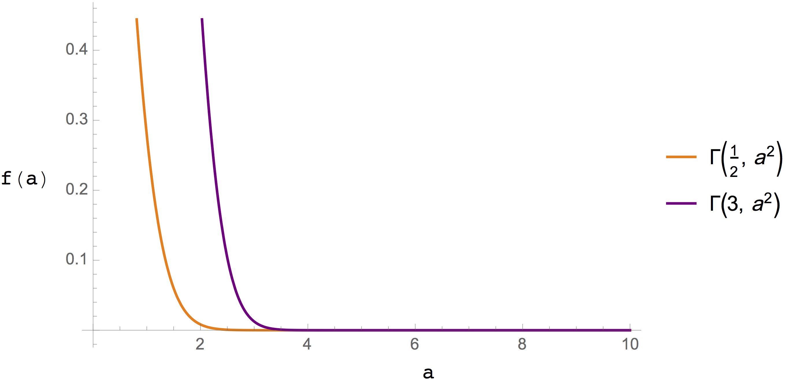
Figure 3. The incomplete gamma function involved in \(U_\mathrm{dir}\) calculations for Coulomb electrostatics (orange line) and dispersion calculations (purple line).

The functions involved in the real- and reciprocal-space summations are graphed in Figure 3. and Figure 4., respectively. In both cases the functions used to evaluate Coulomb and dispersion terms decay rapidly, which is the origin of the improved efficiency.

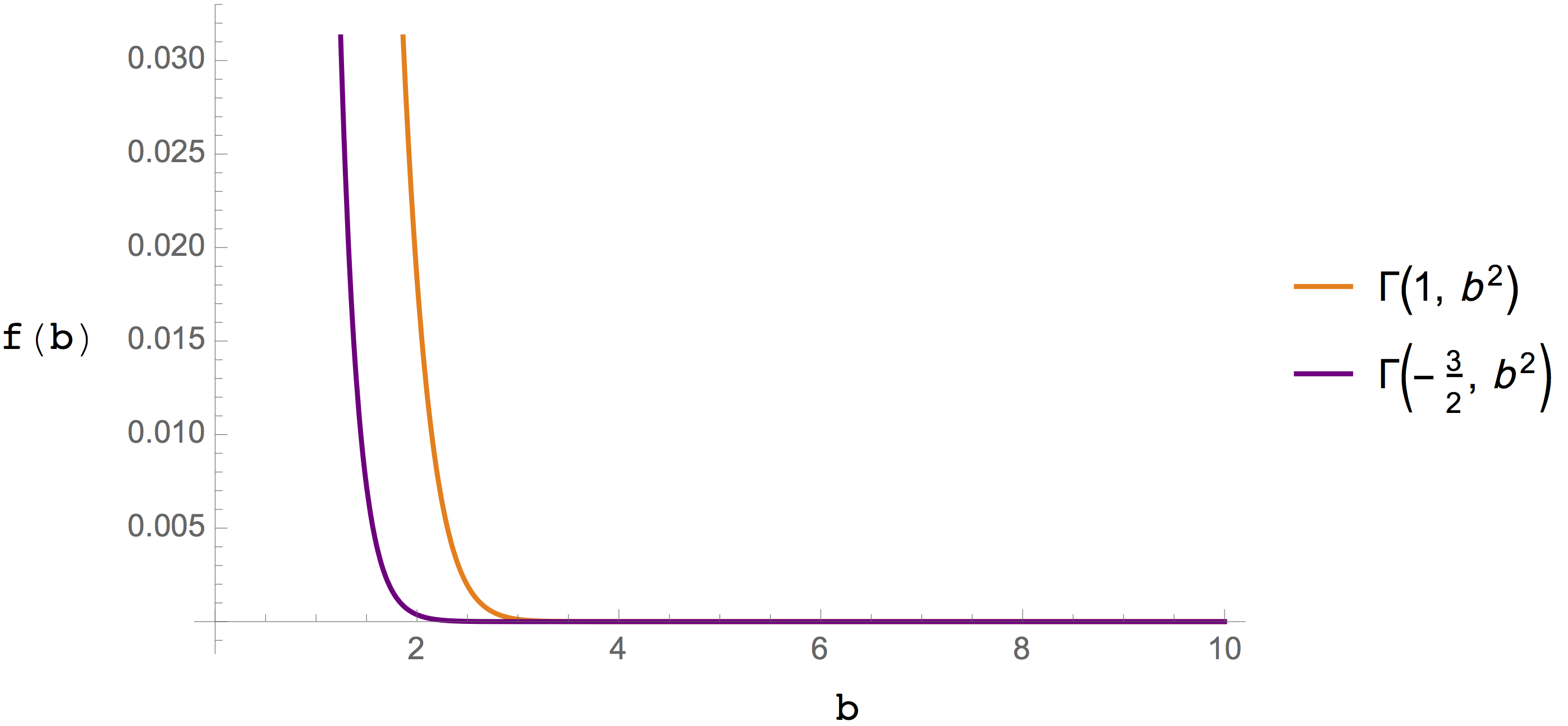
Figure 4. The incomplete gamma function involved in \(U_\mathrm{rec}\) calculations for Coulomb electrostatics (orange line) and dispersion calculations (purple line).

Design Philosophy

The helpme library is designed to be an extensible solution for implementing long range interactions using the \(\mathcal{O}(N \log(N))\) particle mesh Ewald (PME) method.

Boundary Conditions

For kernels with \(1 \leq n \leq 3\), which includes Coulombic systems, the summation is conditionally convergent. In these cases the leading term in the reciprocal space summation is neglected, which corresponds to introducing a neutralizing plasma in charged Coulombic systems. Corrections that reintroduce the conditional convergence, and thus the macroscopic crystal shape dependence, to the PME energy have been developed by a number of different groups. However, for Coulombic systems, these corrections usually depend on the dipole moment of the crystal, which can be discontinuous in systems where a large charge leaves one face of the cell and enters another due to periodic boundary conditions. For this reason, helpme neglects such corrections, which is equivalent to assuming that the crystal resides in a perfectly conducting medium and thus the surface dipole term is zero; this is known as ‘tin-foil’ boundary conditions.

Parallelism

helpme can use MPI to parallelize using 1D-all-to-all variant of the 3D decomposition developed recently in [Jung:2016:57]. The current version of the code assumes that each domain also has coordinate and parameter information for atoms that contribute from neighboring domains; atoms close to domain boundaries contribute to multiple domains. Any atoms present in the list that do not contribute to a given domain are simply filtered out. The full energies, forces and virial can be recovered by a reduction operation involving all domains (MPI tasks). The decomposition imposes the following requirements on the grid dimensions in each direction \(\{n_1, n_2, n_3\}\) and the number of MPI instances in each dimension \(\{P_1, P_2, P_3\}\): \(n_1\) must be divisible by \(P_1\); \(n_2\) must be divisible by \(P_2 \times P_3\); \(P_3\) must be divisible by \(P_1 \times P_3\) and by \(P_2 \times P_3\). The underlying FFT machinery imposes further prime factor constraints for optimal efficiency. Both sets of requirements are automatically satisfied by adjusting the input grid dimension automatically; the actual grid size used is guaranteed to be at least as large as that provided by the caller.

The transforms within a domain are parellelized using OpenMP threading, which is still a work in progress.

Memory

To keep memory usage low, helpme uses a very simple matrix class that allows existing memory to be utilized for forces and coordinates, thus avoiding a copy. All grid-like representations are handled by internally allocating a pool of \(n_1 \times n_2 \times n_3 / P\) complex numbers, split across two bufferes, where \(n_1,n_2,n_3\) are the grid dimensions in each lattice dimension and \(P\) is the total number of MPI nodes. Therefore, per-node memory usage declines as the number of nodes increases.